STAGE II offers the export of content as an image (PNG format), a shapefile for GIS usage (SHP, Esri Shapefile) or a CSV file meant to be imported into data processing programs and spreadsheet programs (Microsoft Excel, LibreOffice Calc). GIS tools also enable the processing tables, which means that STAGE II, in the context of geoinformation processing, offers CSV and SHP files.
In the next step, we will import SHP and CSV files into QGIS. We will transfer a SHP with population density data from 2017 and a CSV with mean age data for the same year. The data is delivered in a ZIP file, which can be extracted with programs such as 7-Zip.
Before importing spatial data, we have to set up the appropriate coordinate system (CRS). Each coordinate system is defined with an appropriate code, called the EPSG code. Some other programs may ask you to define the SRID (Spatial Reference IDentifier) data, which is in this case the EPSG code.
Each country has its own coordinate systems. In the case of using the data of an international criterion, it is reasonable to transform the coordinate systems of all data into reference systems, such as, for example, WGS84 (EPSG: 4326) and ETRS89 (EPSG: 4258). We will tell you more about the transformation of data in the section Data Processing.
Our SHP is given in D48 / GK, EPSG: 3912.
After starting the program, perform the following steps:
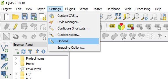
In the coordinate system settings, we have the option of selecting "Automatically enable ‘on the fly’ reprojection” if layers have different CRS”. Choosing this option allows us to properly display spatial data even when we visualize data made in different coordinate systems. This is important only for visualization and does not in any way mean that the data is transformed
We can import spatial data in several ways. We can use the Layer Features -> Insert layer or use their shortcuts, such as  to add vector data and
  to add raster data. In the case that we don’t know the shortcut icons, we can get a description of their function by simply leaving the mouse cursor on them.
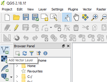
After clicking, a dialog box appears to import the layer. We select our SHP file (a common mistake is click on SHX) and the data is displayed.
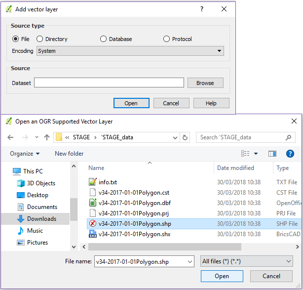
When importing data, a view is loaded, with no special information or colour styles involved. By right-clicking an imported layer we can access the attribute table, where the information our layer contains.
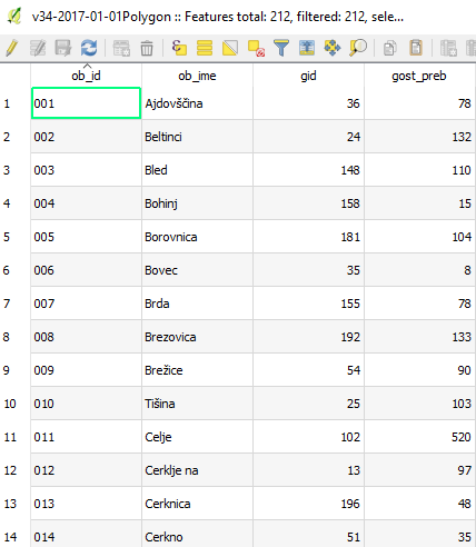
The visualization and processing options of this data will be presented in the following chapters.
We are now proceeding with the import the CSV file. CSV (Comma-Separated Values) is a data format that contains tabular data. As the name suggests, CSV data is, in principle, separated by a comma. In practice they appear separated by different symbols, such as semicolons or tabs. CSV data from STAGE II are separated by tabs because they are way more readable in this form.
We start the import by clicking on the function Add Delimited Text Layer:
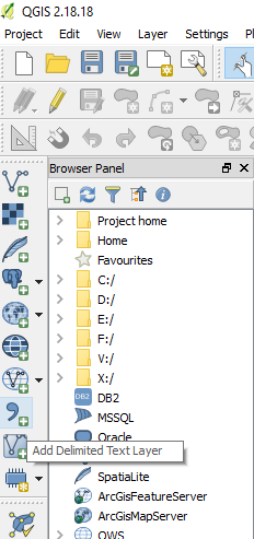
After clicking, a dialog box appears to open the layer. We select our CSV file. In the window below, we have an insight into the data which will be imported and the definition of the structure (with which symbol the data is separated). In our example, we used Custom delimeters and toggled the tab option. Since this CSV has just tabular data and no geometry oene, we must mark No geometry before importing.
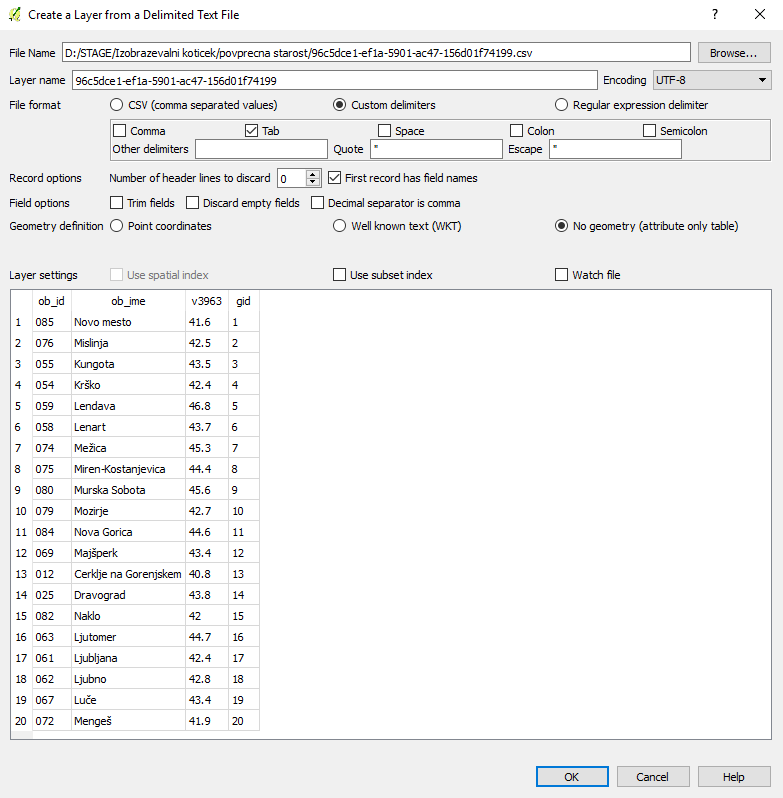
After successfully importing data, we continue with their visualization and processing.